
Introduction
Face morphing is a technique that seamlessly blends two or more facial images to create a smooth transition or a new composite face.
In this project, I will implement the face morphing in 3 stages: Image triangulation, Affine wrapping of the triangles, and Cross-dissolving morphing.
Part 1. Defining Correspondences
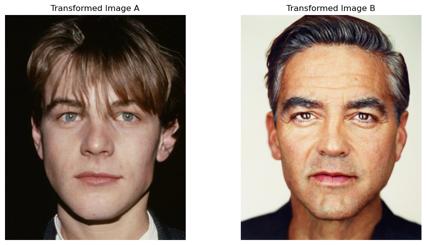
To effectively morph two images, we will need to find the correspondences between the key facial points and then compute a mean shape of the face. To achieve the morphing, we first warp image A into the mean face, then transform from the mean face to image B.
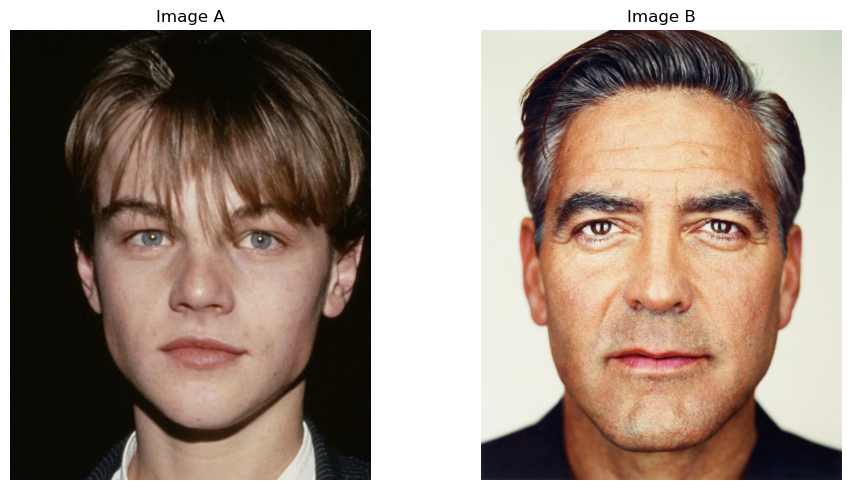
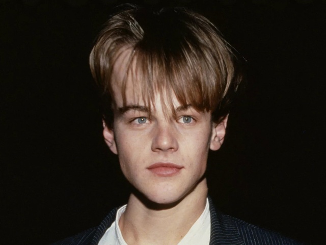
The images I use in this part are A: a random photo of Leonardo, and B: the photo downloaded from the project website.
Initially, we will need to manually annotate the photos with keypoints. I use the following rule to annotate the faces:
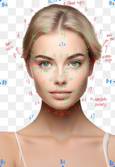
And the result of annotation is shown below:
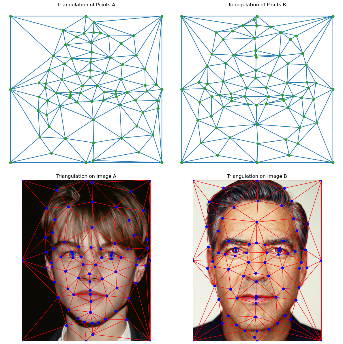
The triangles are computed using scipy.spatial.Delaunay where it aims to maximize the smallest acute angle in each triangle.
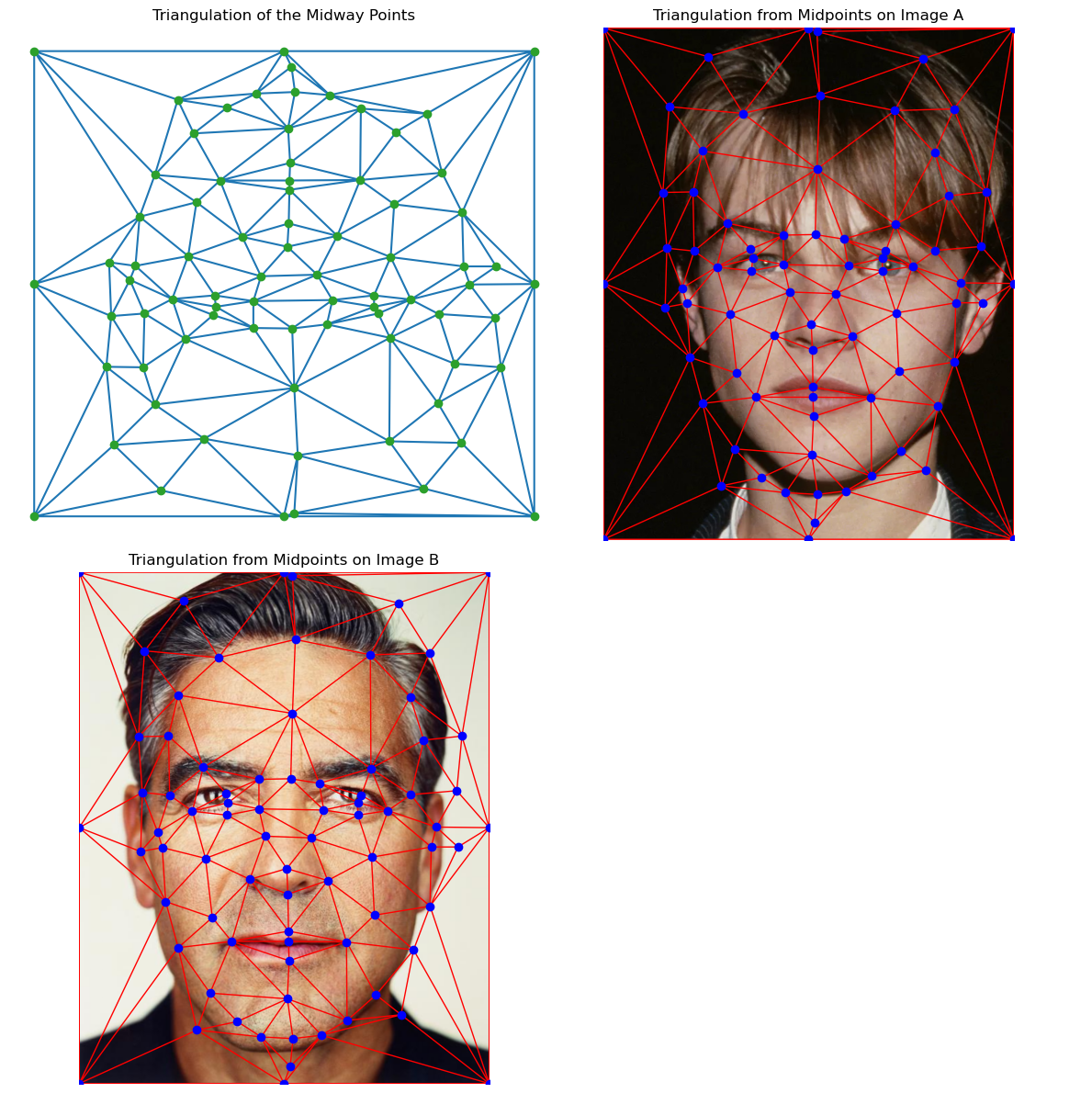
We find the mean face by computing the mean of keypoints:
$$ \text{mean}_{\text{keypoints}} = \frac{1}{2}(\text{keypoints}_{A} + \text{keypoints}_{B}) $$The result of the mean shape:
Since this process is particularly inefficient and tedious, I decided to implement an automatic keypoint annotation model. Check Bells and Whistles for details.
Part 2: Computing the "Mid-way Face"
In this part, I implemented the computeAffine function which, given a list of triangles (obtained from the triangulation in the last part) of the original image, and the triangles of the target image, we compute the affine transformation matrix \(A\) such that \(AP = Q\), where \(P\) is the triangles position matrix (\(3 \times 3\) in homogeneous coordinates), and \(Q\) is the target triangles stacked. \(A\) is an affine transformation, and therefore $$ A = \begin{bmatrix} a & b & c \\ d & e & f \\ 0 & 0 & 1 \\ \end{bmatrix} $$ and $$ A\begin{bmatrix} p^1_x & p^2_x & p^3_x \\ p^1_y & p^2_y & p^3_y \\ 1 & 1 & 1 \\ \end{bmatrix} = \begin{bmatrix} q^1_x & q^2_x & q^3_x \\ q^1_y & q^2_y & q^3_y \\ 1 & 1 & 1 \\ \end{bmatrix} $$ This implies that $$ \begin{bmatrix} p^1_x & p^1_y & 1 & 0 & 0 & 0 \\ 0 & 0 & 0 & p^1_x & p^1_y & 1 \\ p^2_x & p^2_y & 1 & 0 & 0 & 0 \\ 0 & 0 & 0 & p^2_x & p^2_y & 1 \\ p^3_x & p^3_y & 1 & 0 & 0 & 0 \\ 0 & 0 & 0 & p^3_x & p^3_y & 1 \\ \end{bmatrix} \begin{bmatrix} a \\ b \\ c \\ d \\ e \\ f \\ \end{bmatrix} = \begin{bmatrix} q^1_x \\ q^1_y \\ q^2_x \\ q^2_y \\ q^3_x \\ q^3_y \\ \end{bmatrix} $$
In computeAffine, we solve for the coefficients for each corresponding pair of triangles and store them in a list. Then, I implement applyAffine that does the following algorithm:
- Create a meshgrid of \(x\)-\(y\) values, representing the indices of each pixel of the target image. Convert all numbers to the homogeneous coordinate.
- Apply the inverse transform of the affine matrix for each pixel to find the location where it originates before affine transform, effectively avoiding holes. Here, we actually use vectorized code to enhance speed.
- Use bilinear interpolation for each value that lies between pixels.
Then, implement the warp method as follows:
- Compute the triangle masks for each triangle in the target image, using
skimage.draw.polygon. We increase each triangle to be 5% larger (outwards) to create an overlap among triangles and avoid visible borders. - Get the affine transformations from the original image to the target.
- For each triangle, apply the affine transformation on the image, then mask the result with the corresponding triangle mask. Then, use a boolean matrix to override the corresponding portion of the output image.
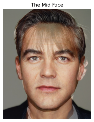
The result of image A and image B warped to their mean shape is:
And their averaged mean face is:
Part 3: The Morph Sequence
In this section, we create a sequence of image morphing and get a smooth transition from image A to image B.
To do this, given total time steps \(n\), and at time \(t\), we compute a warp coefficient \(\phi\) and dissolve coefficient \(\rho\) to be \(\frac{t}{n-1}\). Then, compute the target face to be $$ I_M = (1 - \phi) \cdot I_A + \phi \cdot I_B $$ Then, we warp each image to this middle image, getting \(I_A'\) and \(I_B'\), and mix them according to $$ I = (1 - \rho) \cdot I_A' + \rho \cdot I_B' $$ In this case, at time step 0, the result will be purely image A, and at time \(\frac{n}{2}\), it will be the middle face, and at \(n - 1\), it will be the image B, effectively morphing from A to B.
I collect results for all time steps (n = 45) in order, and play them using fps = 30, and here's the video:
Part 4: The 'Mean Face' of a Population
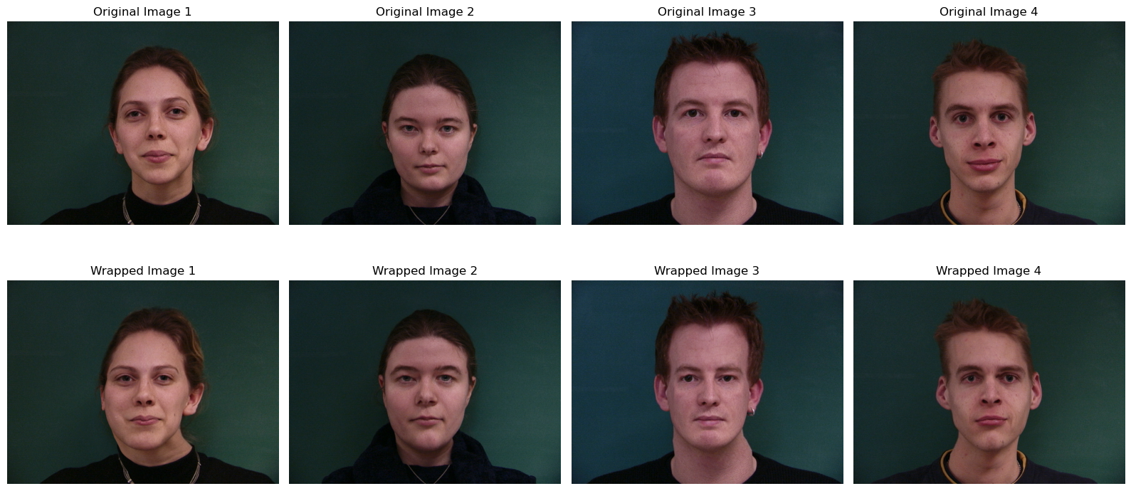
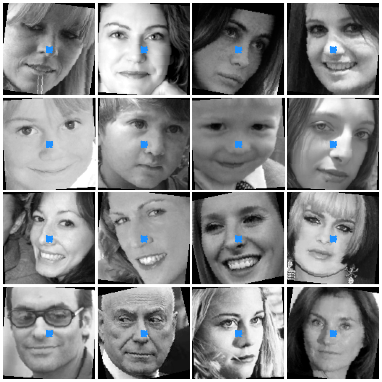
In this section, we will work on this dataset with annotated facial keypoints. Some example keypoints are shown below:
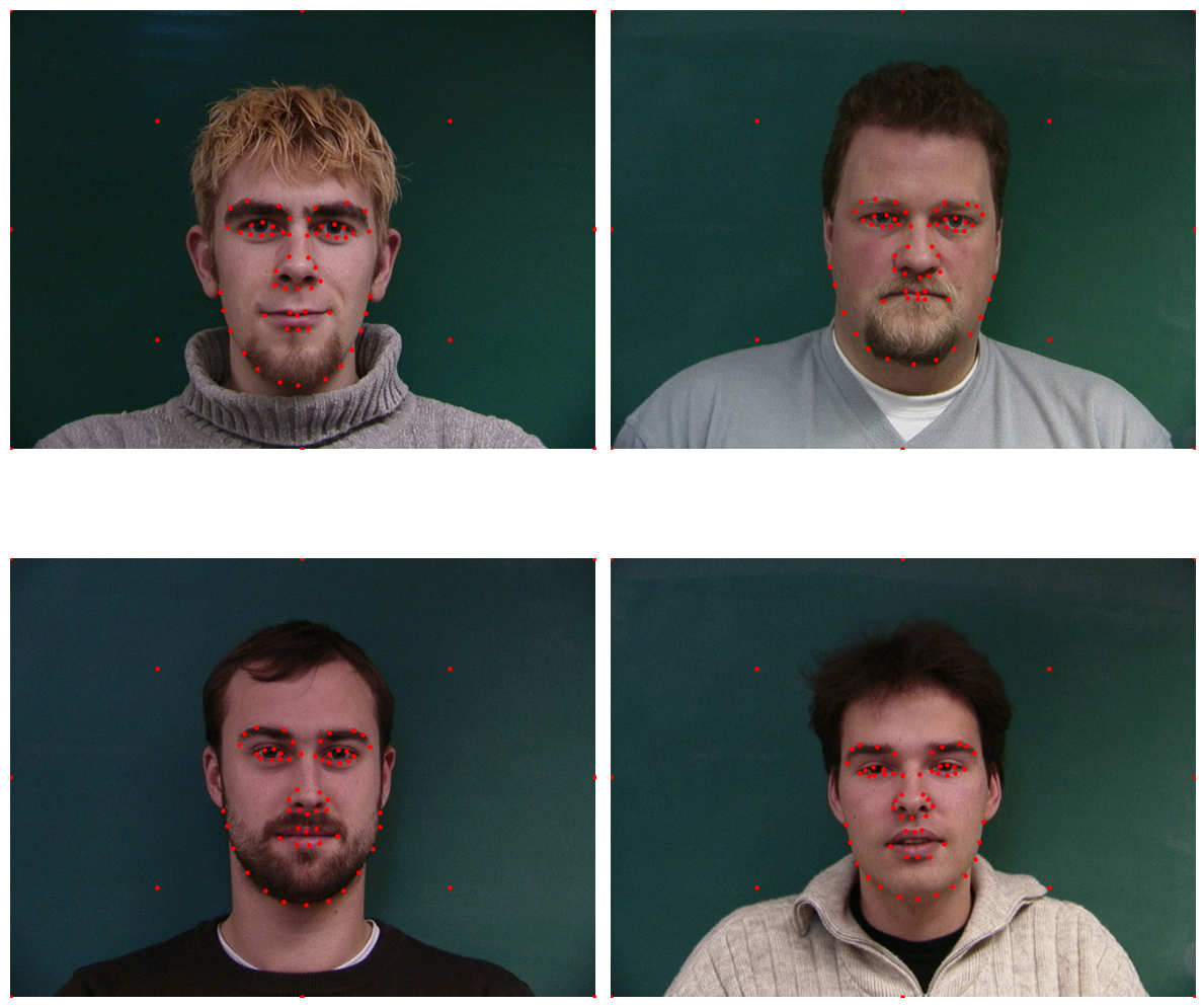
(I add 12 extra points to better warp the backgrounds)
Again, I compute the mean shape of all the points and do a triangulation on that, then warp all images to this mean shape. Some examples are:
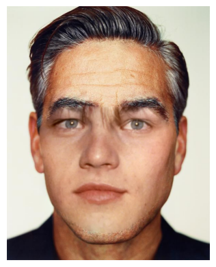
After all images are warped to the same shape, we can compute the mean face:
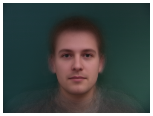
Notice that the skin is smooth, and that's because all the imperfections of the individuals are smoothed out in average.
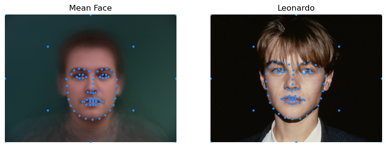
Now, we annotate the previously used photo of Leonardo (using the automatic annotation model I implement in Bells and Whistles):
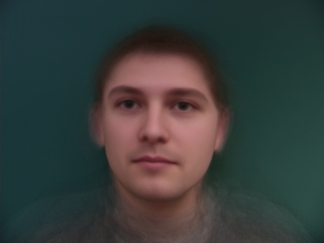
Warping the mean face to Leonardo gives:
Warping Leonardo to the mean face gives:
Part 5: Extrapolation
We can enhance the features of Leonardo's face using the formula enhanced = inverse_warp((1 + alpha) * wrapped_leonardo - alpha * mean_face). When alpha > 1, this is effectively adding the difference between wrapped Leonardo and the mean face multiplied by alpha - 1 to the wrapped Leonardo, and then warp it back to Leonardo's geometry. And when 0 < alpha < 1, it's making Leonardo more towards the mean face. Here are some results:
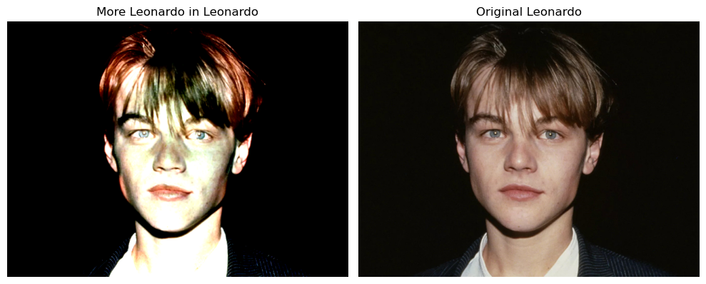
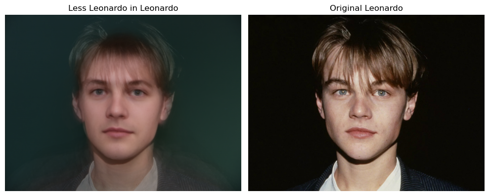
Notice that the enhancing effect is not obvious, and that's because in this picture of Leonardo, he actually looks very similar to the mean face in geometry. Therefore, only color enhancement is obvious. In the Bells and Whistles section, I will try more contrasting mean faces.
Bells & Whistles
Change Gender
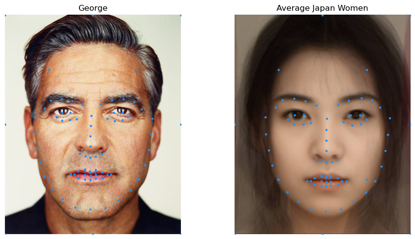
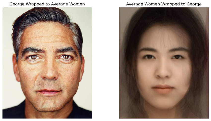
To manipulate the gender, I do the same thing in Part 5 by first warping the target to a mean woman's face, then enhance towards the woman side, and then warp it back. As an example, I make the picture of George more like Japanese women:
Warped towards each other gives:
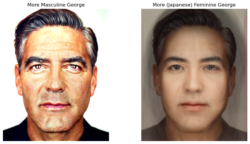
The results of enhancing George towards the feminine side and the masculine side:
Automatic Facial Keypoint Detection Using Neural Nets
In my journey of this project, I found it most painful and boring to manually annotate the points of the face. To correctly warp two images, both the number of keypoints and the order of the keypoints must be the same. To better address this problem and more conveniently annotate the facial keypoints, I use a convolutional neural network to learn on the 300W dataset with around 7000 images and each has 68 keypoints.
Some example keypoints are (these keypoints are annotated labels given along with the dataset):

(The images are converted to grayscale after data preprocessing)
I use the Xception net introduced in this paper, and a brief visualization of the net is:
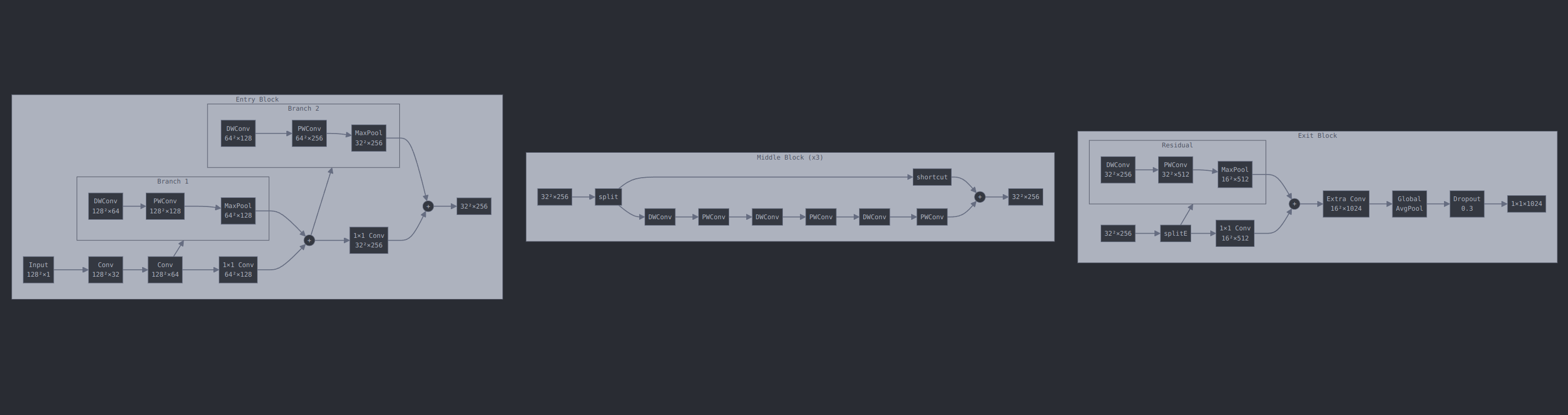
I follow some guidelines from this repo and this paper.
To better generalize on other images, I use data augmentation by randomly rotating, cropping, and offsetting.
Result on the 300W Dataset
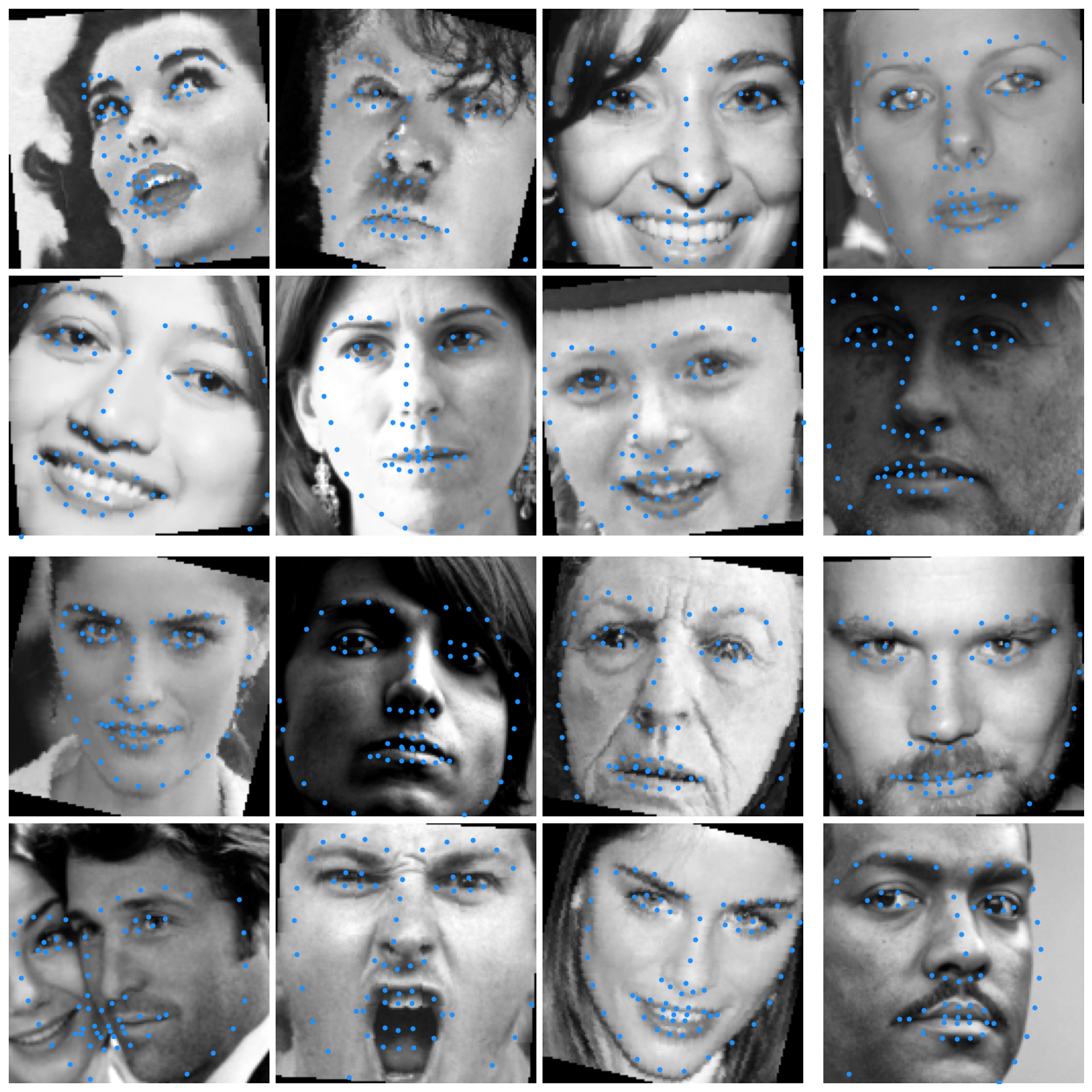
After training 50 epochs on the 300W dataset, the model is capable of annotating facial landmarks with 68 points:
At the beginning, the model gives completely random predictions:
After a few epochs, it starts to learn facial patterns and generates points that look like a face, but not entirely accurate:
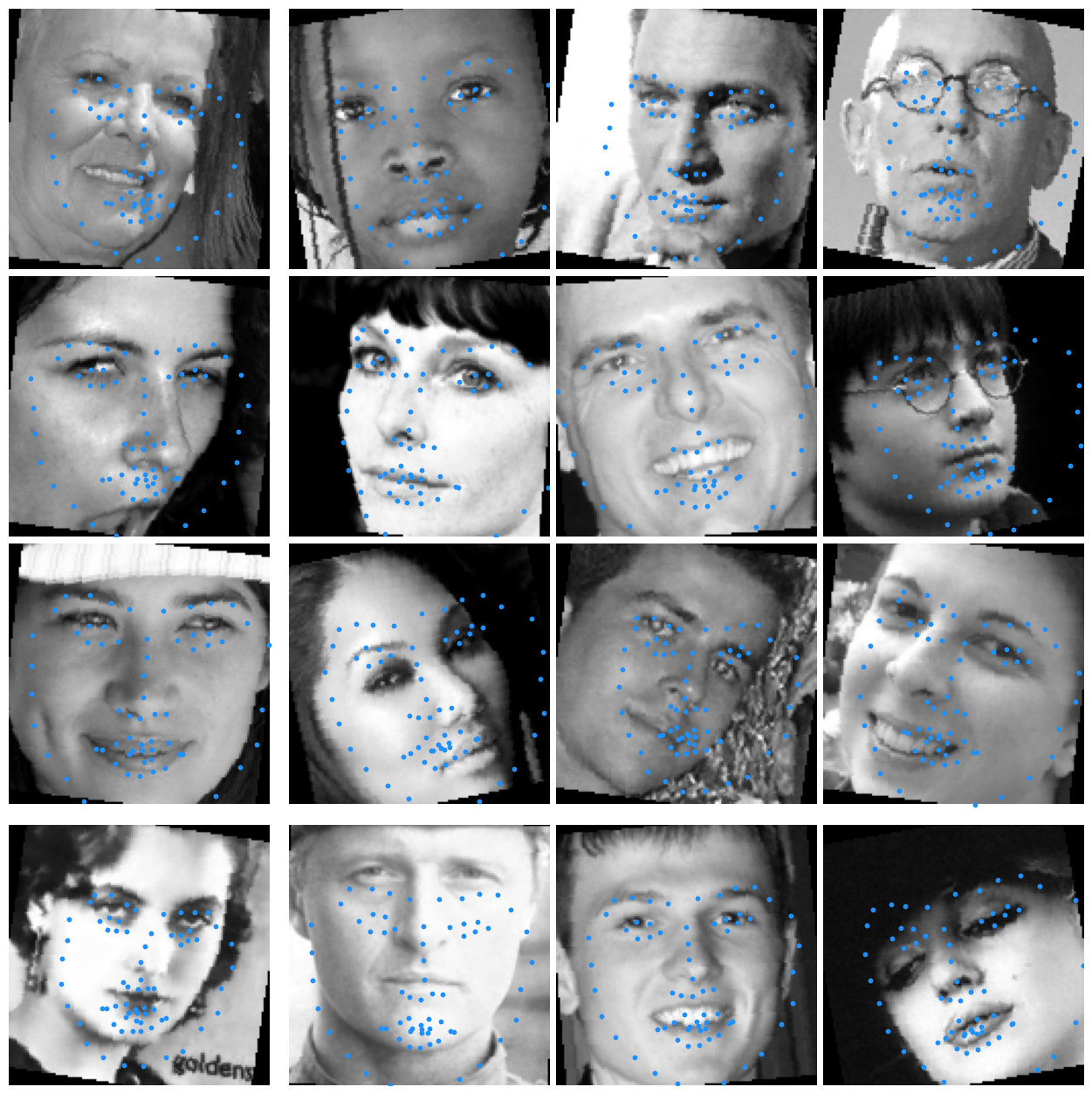
After 30 epochs, the model is capable of predicting almost accurate results on most images:
Transfer Learning on Dane's Dataset
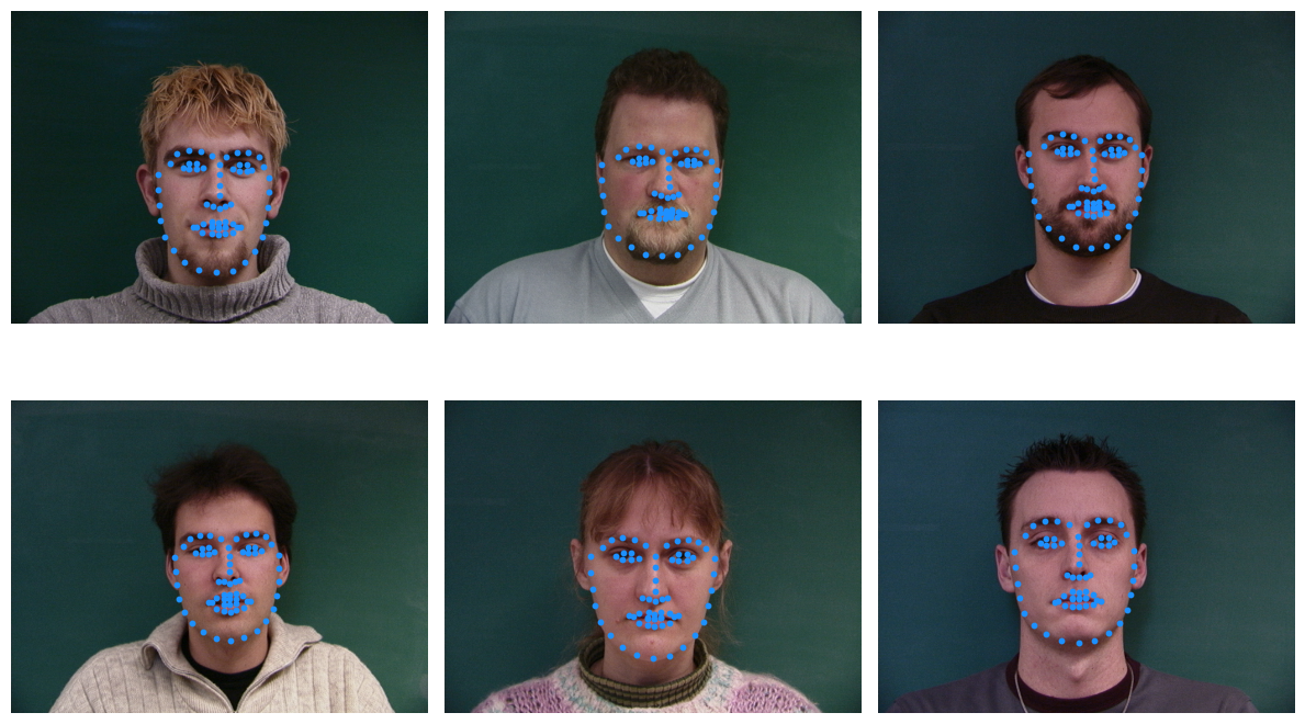
After we have the capable model, we can do cool things like re-annotate the Dane dataset we used in Part 4, and since the 300W dataset has 68 keypoints, it actually provides smoother keypoints on facial landmarks and better morphing performance. Here are some examples of re-annotated Dane datasets:
However, if we want to stick with the original number of keypoints, we can use a trick to convert our learned, 68-keypoints model to a 57-keypoint model that fits the Dane's format. The reason we cannot directly train on Dane is that it's too small (37 images) to get good results. So we do training on 300W first and we remove the fully-connected layer that converts hidden_dim=1024 to output_dim=2*68, and instead make it nn.Linear(1024, 2*57). Then, we freeze the convolutional networks to keep the learned weights safe, and only learn the last fully connected layer. This is called transfer learning.
After doing this for 30 epochs on the Dane dataset, we have a model that predicts keypoints in Dane's format, and here are some comparisons between original keypoints and predicted keypoints:
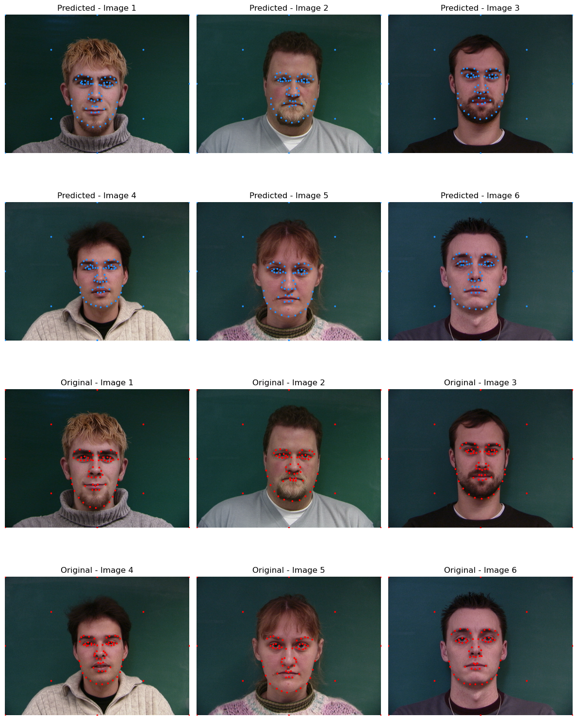
Image Facial Annotation
We can also use the model to annotate each frame in a video:

There are actually keypoints on their faces but the gif is compressed too badly
Face Swap
Given the facial keypoints of two images, we can effectively swap the face of picture 1 tpo picture 2 by applying affine transformation to the region of interests, and mask out other regions.
Here's an example of switching the face of Goerge with Leonardo:
(Implementation of these parts uses high-level functions like OpenCV's ConvexHull, fillConvexPoly, and wrapAffine to handle pictures of difference sizes. I tried to use my customized functions but not working well)